Overview
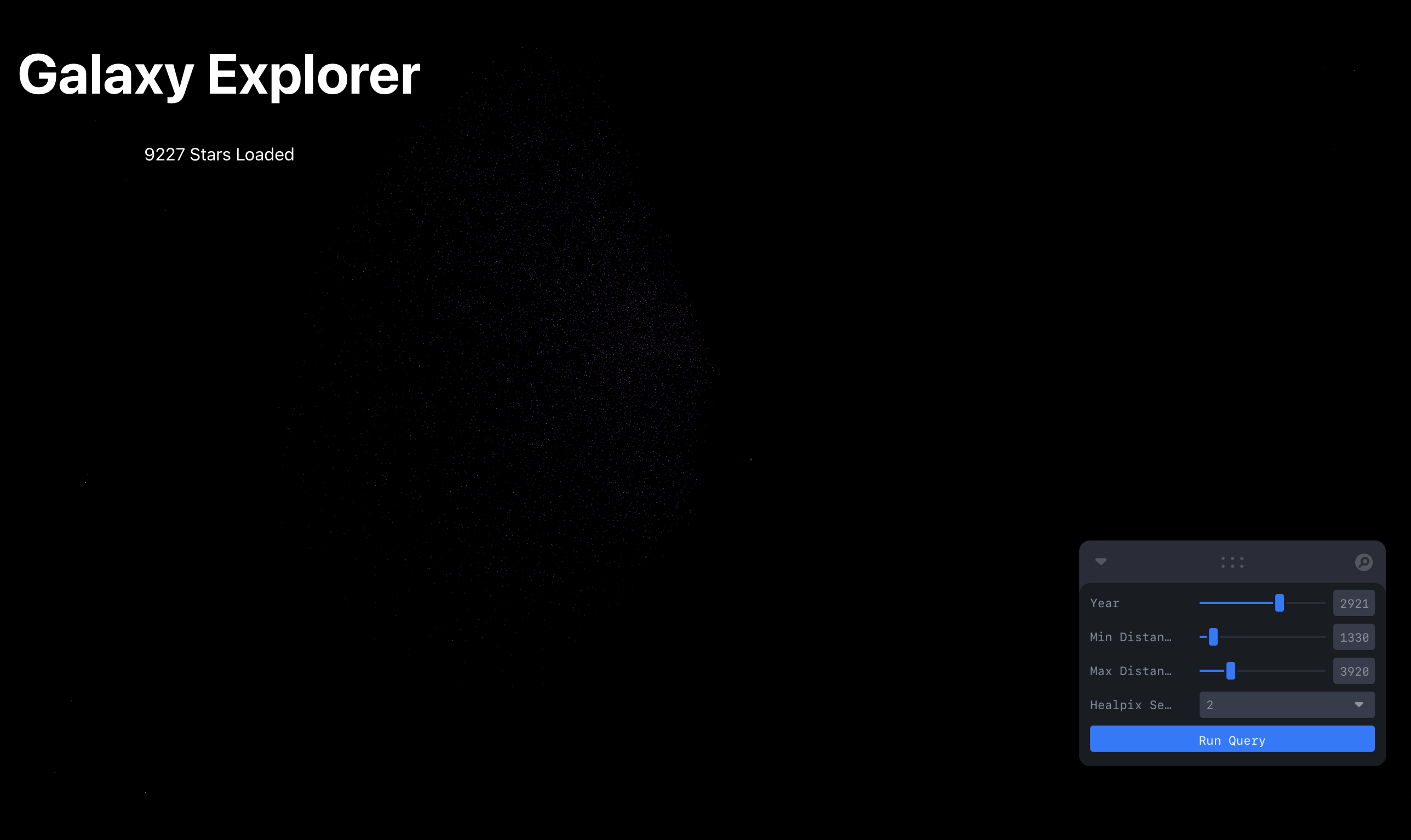
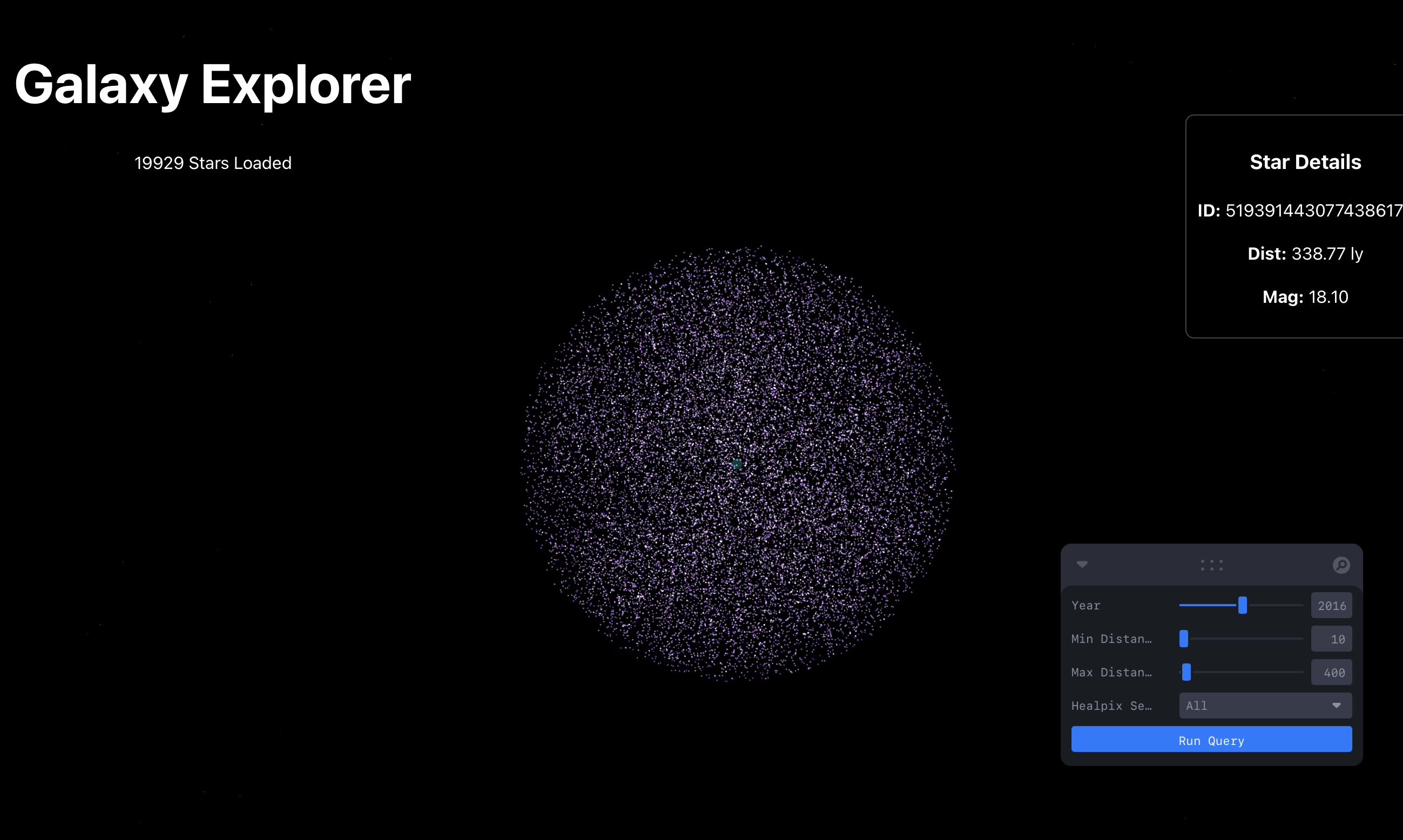
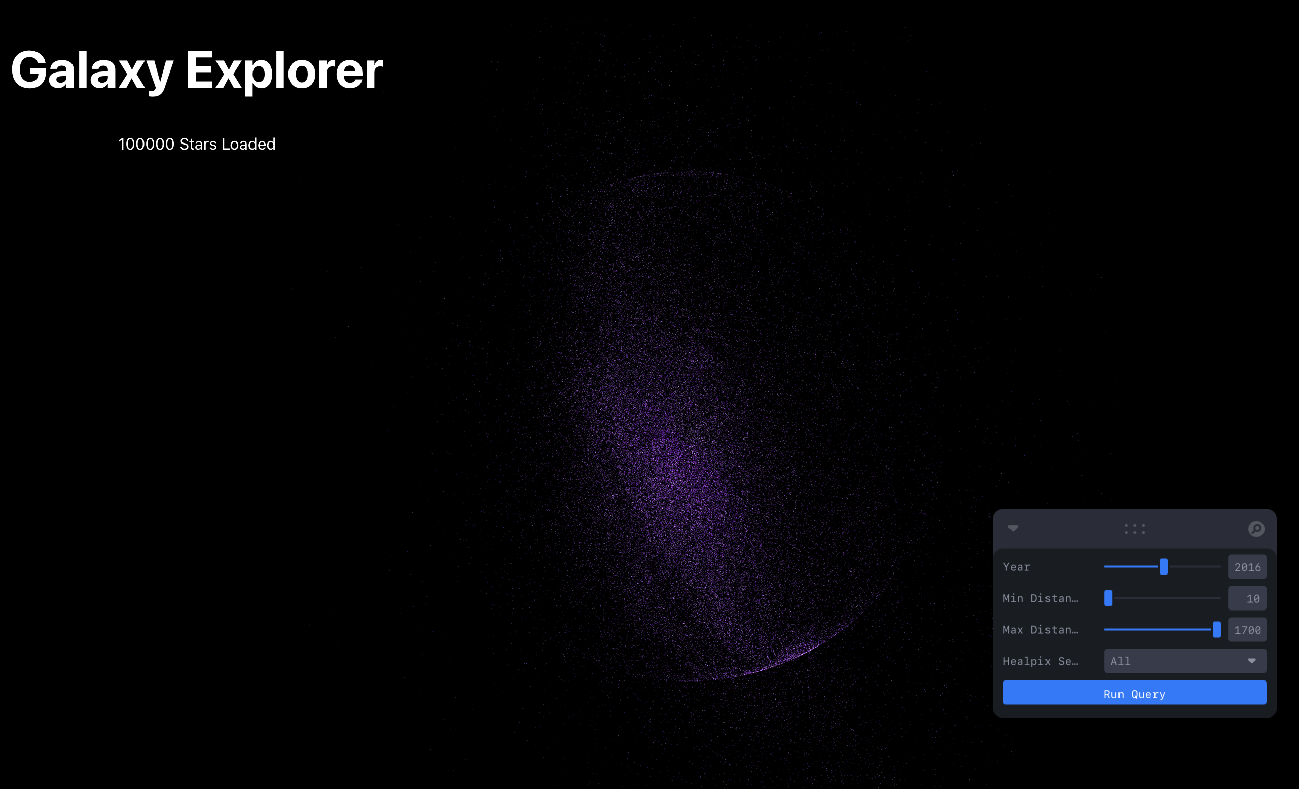
Galaxy Explorer is a cloud-native big-data platform that turns one of the largest scientific catalogues in the world — the European Space Agency's Gaia DR3 star catalogue — into a live, interactive 3D map of the solar neighbourhood. It lets anyone fly through 557 million scientifically validated stars in the browser, scrub the epoch to watch the sky shear over millennia, and run astronomical analytics — stellar density fields, a Hertzsprung–Russell diagram, and unsupervised open-cluster discovery — on demand.
The engineering story is a data-reduction and query-cost story. I started from a raw firehose of roughly 1.8 billion sources, 157 columns and 750+ GB, and engineered it down to a clean, physically meaningful 557 M-star, 13-column serving table — then re-architected the warehouse so that the heavy scan happens once and every interaction afterwards is a cheap, pruned read. The same preprocessing pipeline feeds a second application, a scientifically accurate Night Sky Viewer planetarium, covered at the end of this report. I designed and built the entire system solo, from raw astrometry to a deployed Cloud Run container.
Problem & Goal
Gaia DR3 is a gift and a problem at the same time. It contains positions, parallaxes, proper motions and multi-band photometry for ~1.8 billion stars — but at 750+ GB across 157 columns it is far too large to open in memory, and far too expensive to query naively. Two distinct hard problems follow.
- The data-engineering problem: reduce a 1.8-billion-row, 157-column raw catalogue into a clean, trustworthy, physically meaningful dataset — on a single machine — without ever loading it whole.
- The serving-cost problem: drive interactive 3D exploration and on-the-fly analytics over hundreds of millions of stars from a browser, at low latency and near-zero marginal cost. The naive cloud approach — point a warehouse query at the whole catalogue every time a user moves a slider — full-scans tens of gigabytes per interaction, which is both slow and a real, recurring dollar cost.
The goal was a system where rigour and cost-awareness are designed in from the first byte: a reproducible preprocessing pipeline that shrinks and structures the data, and a warehouse layer that pays the big scan once and then prunes every subsequent query down to only the sky and distance the user is actually looking at.
The Dataset — Gaia DR3
Gaia is an ESA space observatory that has measured the positions, distances (via parallax),
motions and colours of nearly two billion stars. Its third data release, Gaia DR3, is the
backbone of modern Milky Way science. I worked from the full gaia_source catalogue: ~1.8 billion
rows, 157 columns of astrometry and photometry, 750+ GB on disk.
One detail in the catalogue is worth calling out because the whole spatial-indexing strategy hangs on it: Gaia's
64-bit source_id encodes each star's position on the sky. The most significant bits
are the star's HEALPix pixel at level 12, so source_id / 2^35 recovers the level-12 sky pixel with
zero spatial computation, and integer-dividing again rolls that up the HEALPix hierarchy to coarser levels.
That free, baked-in spatial key becomes the partition and clustering column for everything downstream.
| Stage | Sources | Columns | Footprint |
|---|---|---|---|
Raw Gaia DR3 gaia_source | ~1.8 B | 157 | 750+ GB |
| Quality-filtered + feature-engineered (GCS Parquet → external BigQuery table) | 557 M | ~20 | ~77 GB |
| Native serving table — clustered & slimmed | 557 M | 13 | pruned per query |
Data Engineering Pipeline
The reduction from 1.8 billion raw sources to a 557 M-star serving catalogue runs as a multi-stage Polars pipeline. Polars' lazy, multi-threaded, larger-than-memory execution let me process the catalogue one Parquet shard at a time on a single machine — never holding more than a partition in memory — while staying in a columnar format end to end.
Column projection — 157 → ~12
The first and cheapest win is throwing away what I don't need. Of 157 columns, the explorer needs roughly a
dozen — positions (ra, dec), parallax, proper motions
(pmra, pmdec), three-band photometry and source_id. Projecting to those
columns and re-encoding as Zstandard-compressed Parquet collapses the per-row footprint before
any heavy work begins, so every later stage reads a fraction of the original I/O.
Scientific quality filtering — 1.8 B → 557 M
Raw Gaia rows include blended sources, spurious astrometric solutions and contaminated photometry that would poison a 3D map. I apply the community-standard Gaia DR3 quality cuts as a single vectorised Polars mask, keeping only high-confidence stars:
- Astrometric reliability:
RUWE < 1.4(the standard renormalised-unit-weight-error threshold),astrometric_excess_noise < 1,astrometric_sigma5d_max ≤ 2, at least 15 good along-scan observations and at most 5 bad ones, and a valid 5-/6-parameter solution. - Photometric integrity: a flux-over-error floor, caps on contaminated and blended BP/RP
transits, and a quadratic colour-excess mask
(
phot_bp_rp_excess_factor < 1.3 + 0.06·(BP−RP)²) that rejects sources whose colours are corrupted by a nearby neighbour. - Cleanliness: drop duplicated sources, non-single-star solutions, and anything flagged as a quasar or galaxy candidate.
The mask retains roughly 31% of the catalogue — 557 million stars whose positions, distances and colours can be trusted. This is the step that makes everything downstream scientifically defensible rather than just visually plausible.
Spatial indexing with HEALPix
Rather than compute a spatial index, I derive it for free from source_id:
healpix_12 = source_id / 2^35 gives the level-12 pixel, and
healpix_2 = healpix_12 / 4^10 rolls it up to HEALPix level 2 — 192 equal-area sky
sectors. HEALPix (Hierarchical Equal-Area isoLatitude Pixelisation) tiles the celestial sphere into
nested, equal-area cells, so a coarse level-2 sector cleanly contains all of its finer children. I physically
partition the Parquet by healpix_2, so any region-of-sky query reads only the
relevant shards.
Kinematic feature engineering
For 3D rendering and time projection I convert each star from celestial coordinates into a Cartesian state. A
unit direction vector (x, y, z) comes from ra/dec; the physical
distance comes from the parallax (distance_pc = 1000 / parallax in milliarcseconds, then
distance_ly = distance_pc × 3.26156); and a transverse-velocity vector (vx, vy, vz)
is derived from the proper motions pmra and pmdec. Stars with unreliable, near-zero
parallax (< 0.2 mas) are parked at a 10,000-ly sentinel and excluded from analytics, so noisy
distances never reach the map.
Distance binning & aligned partitioning
Finally I bucket each star into a 50-light-year shell
(distance_bin = floor(distance_ly / 50) × 50) and lay the data out by both keys —
sky sector (healpix_2) and distance shell (distance_bin). This is a
deliberate choice: these are the exact two columns BigQuery later clusters on, so the on-disk physical layout and
the warehouse's pruning keys are aligned. A "show me this patch of sky between 200 and 400 ly" query touches a
small, contiguous slice instead of the whole galaxy.
BigQuery: Sub-Second Queries at Low Cost
The processed catalogue lands in Google Cloud Storage as partitioned Parquet, exposed to BigQuery as an external table over ~77 GB / 557 M rows. This is where the project's central engineering problem lives — and the part I'm most proud of.
The clustered native table
External BigQuery tables cannot be clustered, so every query against them full-scans all 77 GB.
The original design also used ORDER BY RAND() to sample stars — meaning each time a user moved the
distance slider, BigQuery scanned the entire 77 GB catalogue at roughly $0.38 per interaction
(on-demand pricing of $5/TB). That is unacceptable for an interactive app.
The fix is a one-time materialisation into a native, clustered, column-slimmed table. I pay the
full 77 GB scan exactly once to build it; from then on, every interactive query prunes by
healpix_2 and distance_bin and reads only the blocks in view:
CREATE OR REPLACE TABLE gaia_ly.stars_native
CLUSTER BY healpix_2, distance_bin AS
SELECT source_id, healpix_2, distance_bin, distance_ly,
       x, y, z, vx, vy, vz,
       phot_g_mean_mag, bp_rp, has_rvs
FROM   gaia_ly.stars            -- external table over ~77 GB of Parquet in GCS
WHERE  distance_ly > 0;
The interactive /stars query then drops ORDER BY RAND() entirely and relies on cluster
pruning plus a LIMIT, so a sector-and-shell request reads a small fraction of the table instead of
all 77 GB. Every BigQuery job in the build is also wrapped in a free dry-run cost estimator that
prints bytes-scanned and a dollar figure before anything executes — cost is a first-class part of the workflow,
not an afterthought.
| Workload | Naive approach | Engineered approach |
|---|---|---|
| Interactive star fetch | external table, ORDER BY RAND() → full 77 GB scan (~$0.38) every interaction | native clustered table pruned by (healpix_2, distance_bin) + LIMIT → a small fraction of 77 GB |
| Stellar density map | GROUP BY over 77 GB, on demand | precomputed density_voxels → kilobytes scanned |
| HR / colour–magnitude diagram | GROUP BY over 77 GB, on demand | precomputed hr_bins → kilobytes scanned |
Precomputed aggregate tables
Analytics that don't need individual stars are pushed into tiny precomputed tables, so the app reads kilobytes instead of re-scanning the catalogue:
density_voxels— one row per (sky sector × distance shell):COUNT(*), mean magnitude and colour, and a flux-weighted centroid (GROUP BY healpix_2, distance_bin). This is the 3D stellar-density field the "Structure" page renders — a whole galaxy's worth of structure in a few thousand rows.hr_bins— a 2D histogram of colour (BP−RP) against absolute magnitude, computed in-warehouse viaabsmag = g − 5·log10(distance_pc) + 5and binned to a 0.05 × 0.2 grid. It powers a live Hertzsprung–Russell diagram in which the main sequence and giant branch emerge straight from the data.
The core result: because external tables can't be clustered, the original design re-scanned
all 77 GB — about $0.38 — on every interaction. Materialising a native table
CLUSTER BY healpix_2, distance_bin turns each interaction into a pruned scan of just the sky
sectors and distance shells in view, and pushing the density map and HR diagram into precomputed aggregate
tables drops those workloads from 77 GB scans to kilobytes.
Stellar Families — HDBSCAN in 6D
The "Families" page finds open clusters and co-moving groups — stars born together that still drift through the galaxy as a pack — with no labels, straight from the data. I restrict to the solar neighbourhood within 600 light-years, where Gaia distances are most reliable and the classic clusters live, and run HDBSCAN over the full 6D phase space: position (x, y, z) and space velocity (vx, vy, vz).
The key insight is that a cluster is defined less by where its stars are than by how they move
together: members share a space velocity to within ~1 km/s while the surrounding field spreads over
~40 km/s. So I standardise position and velocity separately, then up-weight velocity by 3.5×
so shared motion dominates the clustering. HDBSCAN runs with cluster_selection_method="leaf", which
returns the many small, dense knots that are real clusters rather than collapsing them into one giant root blob.
A post-processing pass keeps only genuinely compact groups — rejecting any "cluster" whose positional RMS
exceeds 60 ly or that contains more than 8,000 members as diffuse field — and then auto-labels recovered
groups by matching their centroids against a reference list of famous clusters (Hyades, Pleiades / M45,
Praesepe / M44, Coma Berenices, the Ursa Major moving group, α Persei), with each known cluster naming only its
single nearest match. The output is two native tables — a per-group cluster_catalog and the member
cluster_stars — served to a clickable 3D catalogue in the frontend.
Real-Time Kinematic Projection
Because every star carries a distance and a transverse-velocity vector, the explorer can project the sky to any epoch — letting you scrub forward or backward through time and watch the solar neighbourhood shear. Each star's position at year t is a first-order, constant-velocity propagation from Gaia's reference epoch (J2016.0):
position(t) = direction × distance + velocity × Δt, Δt = t − 2016
The transverse velocity is converted from proper motion in milliarcseconds-per-year into light-years-per-year by
scaling with each star's distance, and the has_rvs flag is carried through to mark the subset with
measured radial velocities. This propagation is done server-side in the API, so the browser
receives ready-to-render points and the projection scales to tens of thousands of stars without bogging down the
client.
Full-Stack System Design
Backend — cloud-native API
The backend is a containerised FastAPI service exposing four endpoints —
/stars, /density, /hr, /clusters — each mapping to one of the
engineered tables. Queries are built with parameterised ScalarQueryParameters (SQL-injection-safe),
and the star sampler uses a density-adaptive LIMIT — more points for wide
distance ranges, fewer per sector — to keep payloads bounded. Crucially, the service
degrades gracefully: if BigQuery or a precomputed table is unavailable, each endpoint falls
back to synthetic mock data, so the UI always renders and local development needs no GCP credentials at all.
Frontend — GPU-accelerated rendering
The frontend is a React + React Three Fiber (Three.js / WebGL) app built with Vite. Tens of
thousands of stars are drawn as a single optimised BufferGeometry particle system, holding a smooth
60 FPS, colour-coded by magnitude, with hover inspection. Two pages sit on the same data layer:
Structure (the 3D density field plus the live HR diagram) and Families (the
HDBSCAN clusters in 3D with a clickable catalogue).
Deployment
Production is a single Docker container on Google Cloud Run: the built React bundle is served by
FastAPI from the same origin as the API, so there is no CORS hop and one stateless service scales horizontally to
zero. The same image runs locally with a MOCK_DATA flag for credential-free frontend development.
Engineering Challenges Solved
- 1.8 billion rows on one machine: the raw catalogue can't be loaded whole. Solved with a shard-at-a-time Polars pipeline in columnar, Zstandard-compressed Parquet — memory stays flat regardless of catalogue size.
- External tables can't be clustered: a 77 GB full scan (~$0.38) on every interaction is a
non-starter. Solved by materialising a native table
CLUSTER BY healpix_2, distance_binso interactive queries prune to the blocks in view. - Re-aggregating the galaxy per request: density maps and HR diagrams don't need raw stars.
Solved by precomputing
density_voxelsandhr_bins, turning 77 GBGROUP BYs into kilobyte reads. - Zero-cost spatial indexing: instead of an expensive spatial join, I exploit the HEALPix
pixel baked into Gaia's
source_idand align the on-disk partitioning with the warehouse cluster keys. - Clusters vs. the field: naive density clustering returns one giant blob. Solved with 6D phase-space features, velocity up-weighting, HDBSCAN leaf selection, and a compactness post-filter that rejects the diffuse field.
- Resilient serving: a missing table shouldn't break the app. Solved with per-endpoint mock fallbacks, so the UI renders and the project is demoable with no cloud at all.
Night Sky Viewer
The second application built on the same Gaia pipeline is a scientifically accurate planetarium. From your latitude, longitude and a draggable time slider, it renders the real sky as a dome (stereographic) projection — true star colours, constellations, the Sun, Moon and naked-eye planets, the Milky Way band, and day/night twilight shading. Its star field is the naked-eye-visible slice of the processed Gaia catalogue (magnitude ≤ 6.5), cross-matched with the HYG database for proper names and Bayer designations and d3-celestial for constellation lines and the Milky Way outline.
The astronomy is real, not decorative. A dedicated skyview package converts equatorial RA/Dec to
horizontal altitude/azimuth with vectorised NumPy via local sidereal time, applies a Bennett
atmospheric-refraction term near the horizon, and propagates each star's position from the
J2016.0 epoch using its Gaia proper motion. Sun, Moon and planet positions, the Moon's illuminated phase and the
twilight state come from astropy with bundled ephemerides and IERS tables, so the deployed app
needs no network at runtime. Star colours are physical: a colour index is mapped to an
effective temperature (Ballesteros relation), then to an sRGB blackbody tint — hot stars blue-white, Sun-like
stars yellow, cool stars orange-red.
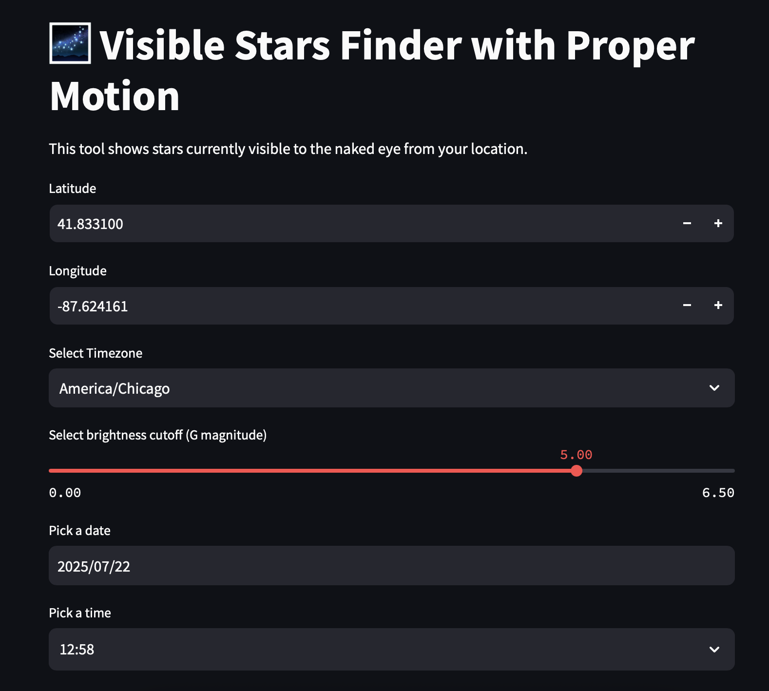
A magnitude slider (6.5 for dark rural skies down to ~2 for bright urban skies) lets you simulate light pollution, city presets and one-tap GPS set your location, and a time-lapse "play" mode advances the clock so you can watch the whole sky rotate.
Tech Stack
- Data engineering: Polars (larger-than-memory, shard-at-a-time processing), NumPy, Zstandard-compressed Parquet, HEALPix spatial indexing.
- Warehouse: Google BigQuery (external tables, native clustered tables, precomputed aggregates, dry-run cost estimation), Google Cloud Storage data lake.
- Machine learning: HDBSCAN 6D phase-space clustering, scikit-learn (
StandardScaler). - Backend: FastAPI, Uvicorn, Pydantic, the BigQuery Python client with parameterised queries.
- Frontend: React, React Three Fiber, Three.js (WebGL), Vite, Axios.
- Planetarium: Streamlit, astropy (ephemerides, sidereal time, refraction), NumPy; HYG and d3-celestial overlays; SIMBAD / Hipparcos / Tycho-2 cross-matching for names.
- Infrastructure: Docker, Google Cloud Run (single-container deploy), graceful mock-data fallback for credential-free local dev.
Outcomes & Impact
- Engineered a 750+ GB, ~1.8-billion-source, 157-column raw Gaia DR3 catalogue down to a clean, physically meaningful 557 M-star, 13-column serving table — entirely on a single machine.
- Cut interactive query cost from a ~77 GB / ~$0.38 full scan on every interaction to cluster-pruned reads, and pushed density and HR analytics into precomputed tables scanned in kilobytes.
- Made 557 M+ stars explorable in 3D at 60 FPS in the browser, with server-side epoch projection for travelling through time.
- Recovered known open clusters and moving groups — Hyades, Pleiades, Praesepe, Coma Berenices and more — unsupervised, via 6D HDBSCAN in position + velocity.
- Shipped the whole system as a single Cloud Run container with resilient mock-data fallbacks, plus a second app — a scientifically accurate Night Sky planetarium — on the same pipeline.
Conclusion
Galaxy Explorer is the project I point to when I want to show that I can take a genuinely large scientific dataset and engineer it all the way to a fast, cheap, interactive product. It pairs the data engineer's instincts — shrink the data, structure it around how it will be queried, and make the warehouse pay the big scan only once — with the discipline to keep every number scientifically defensible and the cost of every query visible. From 750 GB of raw astrometry to a 3D galaxy you can fly through in a browser, it's the clearest demonstration of how I think about big data: not as something you scan, but as something you design.