Traffic Prediction

Overview

This project forecasts traffic conditions and generates optimized travel routes using a Random Forest Regressor for prediction and Dijkstra’s algorithm for route planning. To improve accuracy, it incorporates real-time and historical traffic data, along with roadblock and accident reports scraped from news websites using the Beautiful Soup library. Interactive route visualizations are created with Folium.

Data Preprocessing

The dataset used in this project was the CalTrans traffic dataset for the city of San Francisco. Key steps in preprocessing included:

• The raw data came as multiple text files — one per day — sampled every 5 minutes.
• Regex was used to extract relevant information and compile it into a pandas DataFrame.
• Main columns included: date, time, section, district, lane, flow, and others.
• A specific region within San Francisco was filtered for focused analysis.
• Missing values were handled using a KNN imputer.
• The final dataset consisted of 315,359 entries, representing approximately 3 years of data.

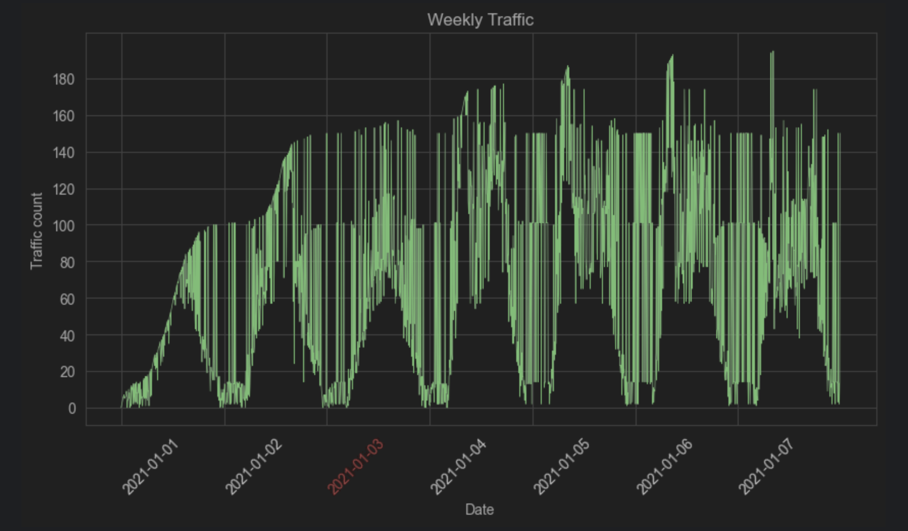
This image illustrates the daily traffic patterns in San Francisco. Dates highlighted in red represent Sundays. The data reveals a consistent trend across all days: traffic volume increases in the morning, peaks around midday, and gradually declines afterward — regardless of whether it’s a weekday or weekend.

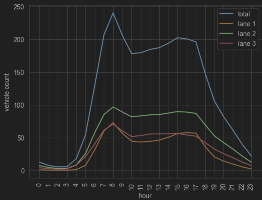
This image displays the hourly traffic volume across different lanes. The graph shows two distinct peaks — one in the morning and another in the evening — reflecting typical commute times during standard working hours.

Approach

We began by experimenting with ARIMA models, which are well-suited for capturing patterns in time series data. However, due to the high frequency and complexity of the dataset, even advanced ARIMA configurations struggled to accurately model the traffic trends.

As a result, we shifted to a machine learning-based approach. Temporal features such as minute, hour, and day of the week were extracted and included as model inputs to better capture periodic patterns.

We evaluated three primary models based on the nature of the data:

• Polynomial Regression
• Ridge Regression
• Random Forest Regressor

Among these, the Random Forest Regressor outperformed the others, offering the best balance of accuracy and generalization for our traffic prediction task.

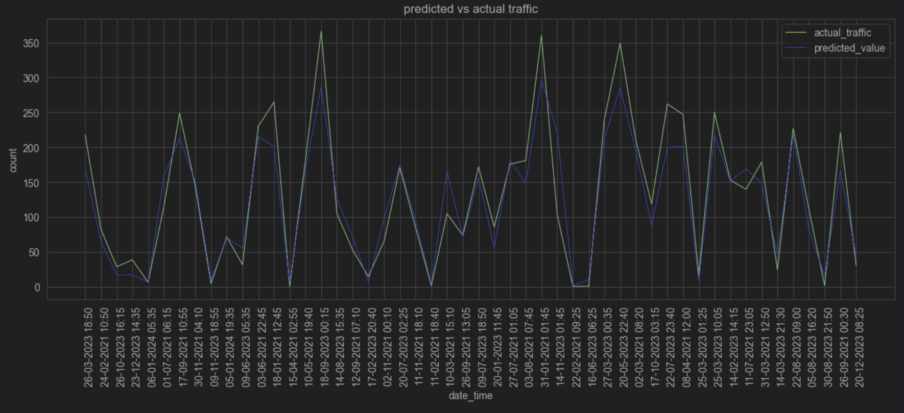
As shown in the image, the predicted values closely align with the actual traffic data. While the model slightly overfits in certain regions, it still struggles to predict extreme values accurately. These outliers were not removed, as they may correspond to special events or public holidays in the city. In future iterations, we plan to include such contextual factors as additional features to improve the model's performance.

Web Scraping

To account for external factors that could impact traffic patterns — such as city events, road closures, or accidents — we utilized information from local news websites. Using the Python library BeautifulSoup, we performed web scraping to extract relevant updates that could serve as contextual features in our model.

Maps

We integrated the model predictions and event data from web scraping into a weighted graph network, where edge weights reflect traffic conditions. This network allows us to compute the most efficient routes across the city.

For pathfinding, we initially implemented Dijkstra’s algorithm. While effective, it can become computationally expensive for larger graphs — in such cases, A* search serves as a more scalable alternative.

To accurately compute distances between geographic points, we used the Haversine formula, which accounts for the Earth's curvature based on latitude and longitude.

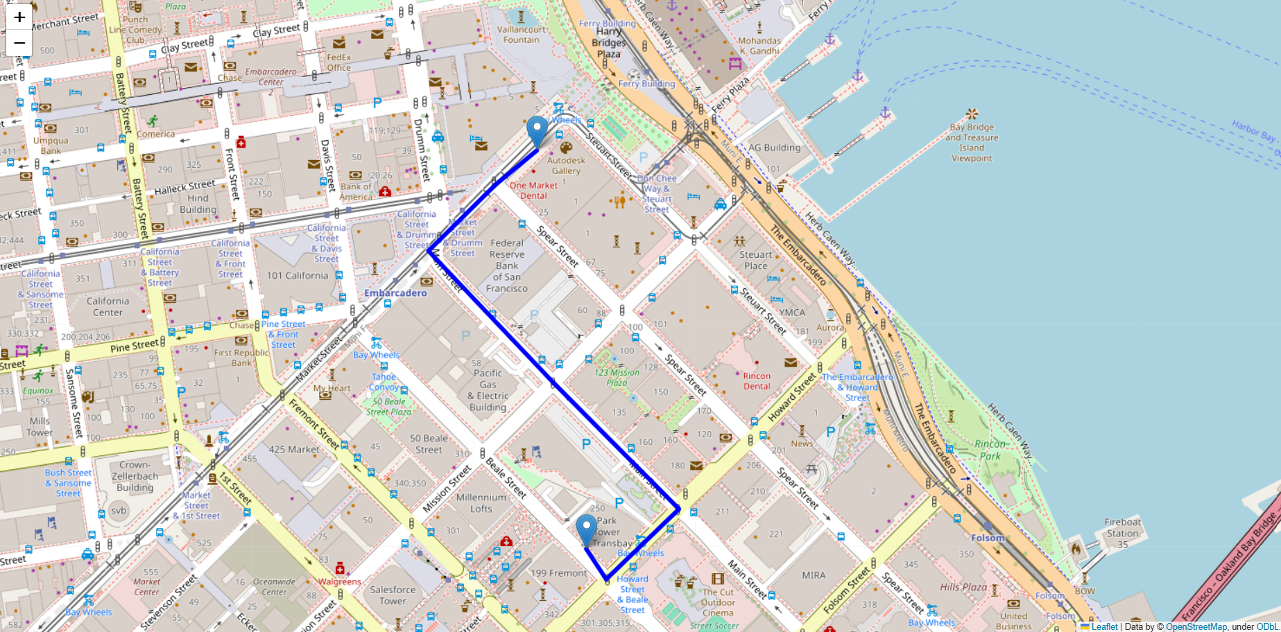
The final output is visualized using Folium maps, displaying the predicted shortest path between two selected locations.

Conclusion

This project provided valuable hands-on experience in preprocessing and modeling time series data, as well as a deeper understanding of the challenges involved in making accurate predictions. It also allowed me to explore and apply lesser-known Python libraries, contributing to a more comprehensive and well-rounded solution.