Alzheimer's Progression · Madhu Siddharth Suthagar

Overview

Alzheimer's Progression is an end-to-end deep-learning system that does two things from a single brain MRI slice: it stages the disease and it shows you what comes next. A fine-tuned EfficientNetB4 classifier reads a scan and assigns it to one of four clinical stages, and a chain of three DCGANs then synthesizes how that same brain is likely to look as the disease advances — turning a one-off diagnosis into a visual prognosis. The whole pipeline is wrapped in a Flask web app, containerized with Docker, and instrumented with MLflow so every training run is reproducible.

The system is trained and evaluated on the OASIS MRI dataset — 86,437 labelled slices spanning Non Demented, Very Mild, Mild, and Moderate dementia. The classifier reaches 98% accuracy (0.98 macro-F1) on a held-out test set, and adding region-of-interest guidance to the generators cut their FID by ~23%, producing noticeably sharper, more anatomically faithful progression images. It was built as a team project for CS 584 (Machine Learning), and it deliberately spans the full arc — data analysis, transfer learning, generative modeling, and deployment — rather than a single notebook.

Problem & Motivation

Alzheimer's disease is progressive and irreversible, and the window where intervention helps most is early — precisely when the structural changes on an MRI are subtlest and easiest to miss. Two distinct machine-learning problems follow from that. The first is diagnostic: given a scan, which of the four stages is this? The second is prognostic and far harder: can we make the likely future of a specific brain visible, so a clinician or patient can see the trajectory rather than read a label off a chart?

We tackle both, and we do it on top of a genuinely difficult dataset. Real medical imaging is brutally imbalanced — healthy scans vastly outnumber late-stage ones — and the visual gap between adjacent stages is small enough that even the difference between two stages is mostly low-contrast structural drift. The goal was never just a model file; it was a defensible system that classifies accurately and generates progression imagery a non-specialist can actually interpret.

Dataset & Exploratory Analysis

The foundation is the open OASIS MRI dataset: 86,437 axial brain slices labelled across four Alzheimer's stages. As is typical of clinical data, the distribution is severely skewed — Non Demented scans outnumber Moderate Dementia scans by roughly 138 to 1, which dominates every downstream design decision from sampling strategy to how we report metrics.

Stage	Images	Share of dataset
Non Demented	67,222	77.8%
Very mild Dementia	13,725	15.9%
Mild Dementia	5,002	5.8%
Moderate Dementia	488	0.6%
Total	86,437	100%

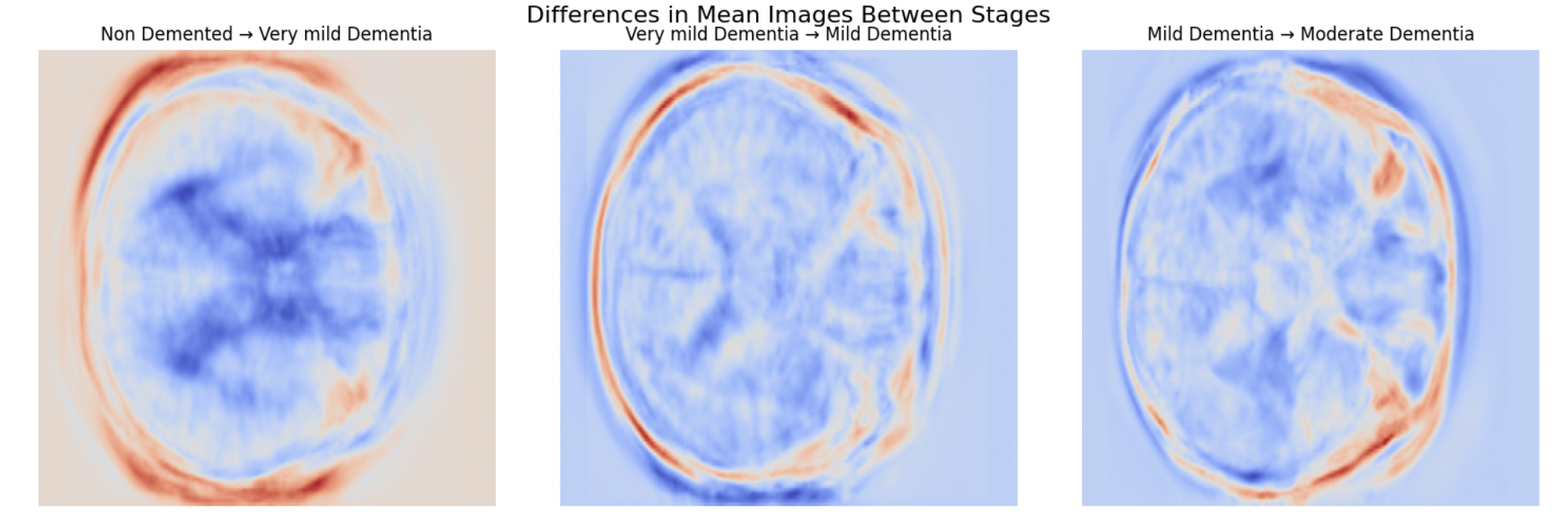
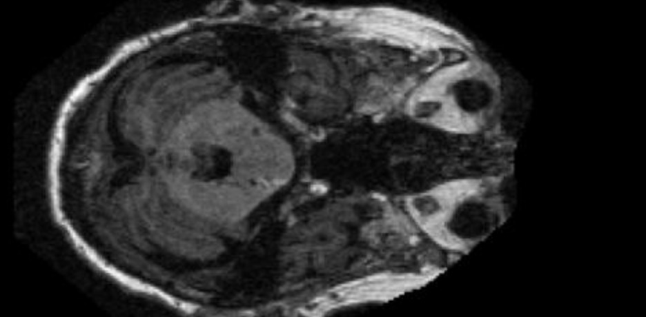
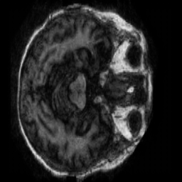
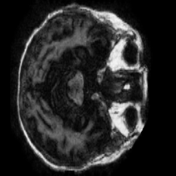
Before modeling, we ran a focused EDA to understand where and how the disease shows up on a scan. Averaging every image within a stage and subtracting consecutive means produces a difference map that localizes change: the recurring signatures are cortical thinning at the brain's periphery and ventricular enlargement toward the centre — spatially consistent across patients, which is exactly the kind of structure a generator should learn to reproduce.

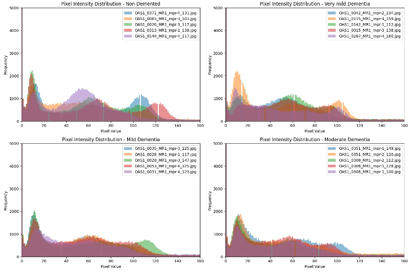
Difference in mean images between consecutive Alzheimer's stages — Figure 1 — Mean-image difference maps between consecutive stages (Non→Very Mild, Very Mild→Mild, Mild→Moderate). Warm and cool regions mark where structure changes most as the disease advances.

We also profiled pixel-intensity distributions per stage. Healthy brains show distinct frequency spikes around the 40–60 and 100–140 intensity bands; as the disease progresses these distributions flatten, signalling a loss of contrast and structural definition. That finding mattered for the GANs: without careful normalization, a pixel-level generator will happily learn brightness shifts instead of the anatomical changes that are actually clinically meaningful, so every image is normalized before it reaches a model. A complementary SSIM analysis between adjacent stages confirmed how structurally similar neighbouring stages are — quantifying why this is a hard, fine-grained problem rather than a coarse one.

Pixel intensity distributions across stages — Figure 2 — Per-stage pixel-intensity histograms. The characteristic spikes in healthy scans flatten as dementia advances, motivating intensity normalization before generation.

System Architecture

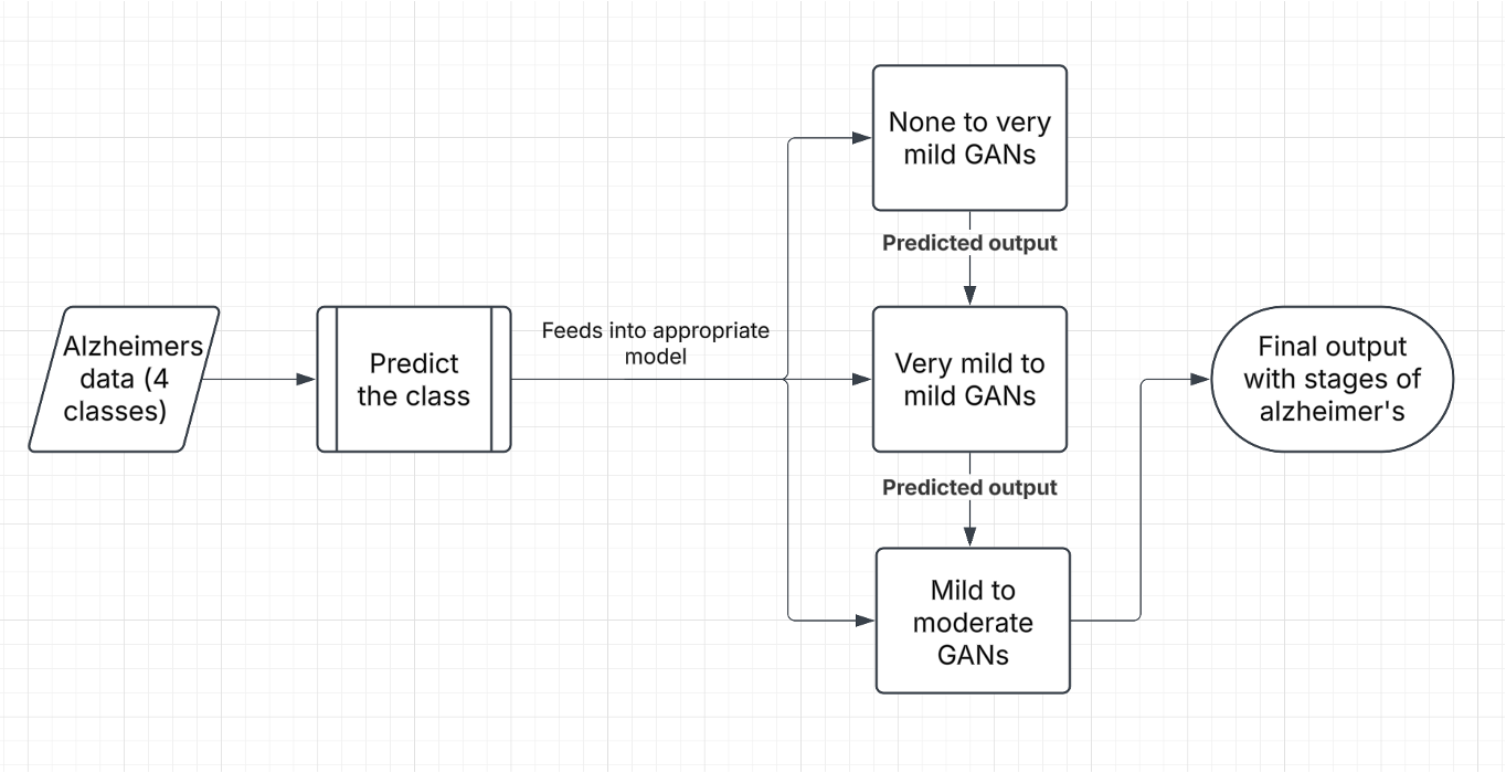
The pipeline is two models working in sequence. An incoming MRI is first resized and converted to RGB, then passed to the EfficientNetB4 classifier, which predicts the current stage. That prediction acts as a router: the scan is fed into the generator trained for its specific stage transition, and the generators are chained — the output of one becomes the input of the next (Non→Very Mild→Mild→Moderate) — until the brain reaches the final stage. The result returned to the user is the predicted current stage plus a sequence of synthesized scans illustrating the road ahead.

End-to-end architecture: classifier routes into a chain of stage-transition GANs — Figure 3 — End-to-end architecture. The classifier predicts the stage, which selects an entry point into the chained stage-transition GANs that generate the remaining progression.

Stage Classifier — EfficientNetB4

The classifier is built on EfficientNetB4 pre-trained on ImageNet, with its default head replaced by a single dense layer mapping to our four stages. Inputs are 256×256 and standardized with ImageNet statistics; training uses light, anatomy-preserving augmentation — horizontal flips, ±15° rotations, and mild brightness/contrast jitter — on an 80/20 train/validation split, optimized with cross-entropy.

The key choice is a two-phase transfer-learning schedule. In Phase 1 the entire backbone is frozen and only the new classification head is trained (Adam, learning rate 1e-3, 10 epochs), so the freshly initialized head adapts without destroying ImageNet's learned features. 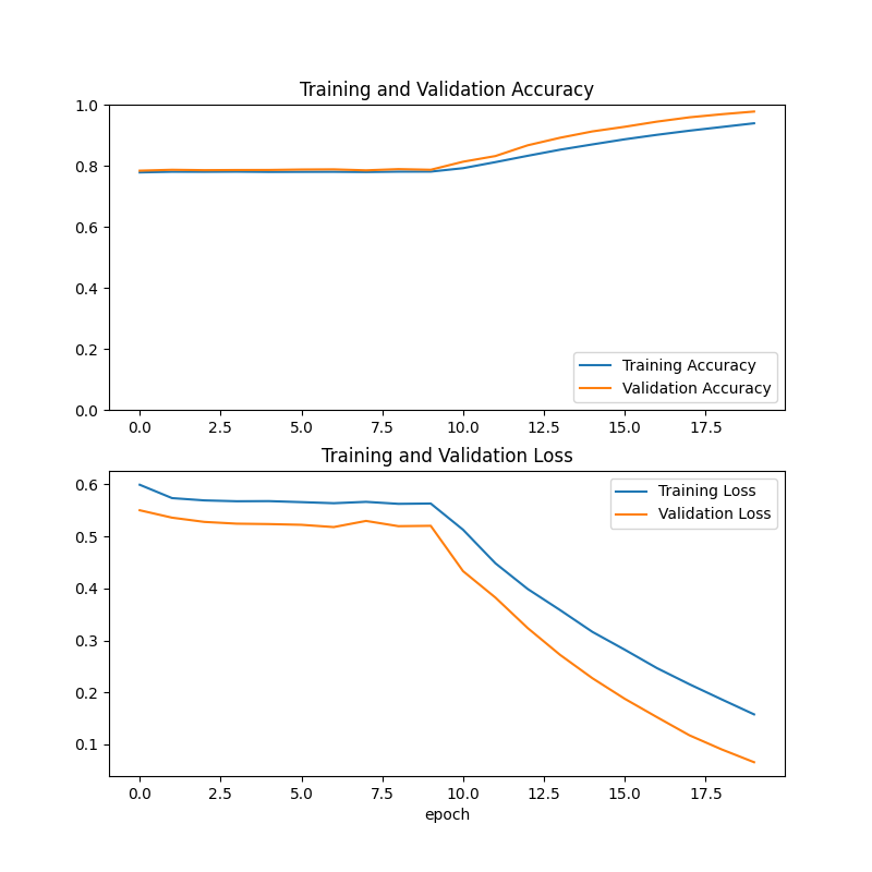In Phase 2 every layer is unfrozen and the whole network is fine-tuned at a far gentler rate (Adam, 1e-5) under a ReduceLROnPlateau scheduler, with the best-validation checkpoint kept. The training history makes the payoff obvious: accuracy sits flat around 78% while the backbone is frozen, then climbs sharply to ~98% the moment fine-tuning begins, as validation loss falls from ~0.55 to under 0.10. Training runs on Apple Metal (MPS) or CUDA when available.

Training and validation accuracy and loss across the two-phase schedule — Figure 4 — Two-phase training history. Accuracy is flat (~78%) while the backbone is frozen and jumps to ~98% once fine-tuning unfreezes the network around epoch 10; loss falls in lockstep.

Classification Results

Evaluated on a 2,048-image held-out set drawn from the natural (imbalanced) distribution, the fine-tuned model reaches 98% overall accuracy with strong per-class precision and recall:

Stage	Precision	Recall	F1-score	Support
Non Demented	0.99	0.99	0.99	1,588
Very mild Dementia	0.96	0.94	0.95	333
Mild Dementia	0.98	0.98	0.98	117
Moderate Dementia	1.00	1.00	1.00	10
Accuracy	0.98			2,048
Macro avg	0.98	0.98	0.98	2,048
Weighted avg	0.98	0.98	0.98	2,048

The headline isn't just the 98% accuracy — on an imbalanced set, accuracy flatters a model that only nails the majority class. The more honest signal is the 0.98 macro-averaged F1, which weights every stage equally: even Very Mild (the subtle, easy-to-confuse stage) holds a 0.95 F1. The one figure to read with care is Moderate Dementia, whose perfect scores rest on only 10 test images — a direct consequence of how rare that class is in the source data.

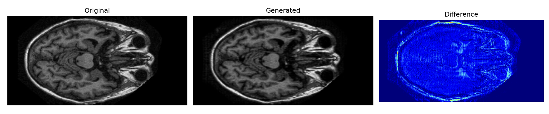
Progression Modeling with DCGANs

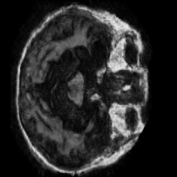
Generating the future of a brain is framed as image-to-image translation, not noise-to-image synthesis: each generator takes a real scan at one stage and produces the corresponding scan at the next. We train three separate DCGANs, one per transition — Non→Very Mild, Very Mild→Mild, and Mild→Moderate — all sharing the same architecture.

The Generator is an encoder–decoder convolutional network. Three strided convolutions (kernel 4, stride 2) downsample the single-channel input into 256 feature maps with ReLU activations and batch normalization, and three transposed convolutions upsample back to a one-channel image, ending in a Tanh that maps pixels to [-1, 1] — letting the network learn detailed pixel-level transformations between stages. The Discriminator mirrors it: four convolutional layers with LeakyReLU (slope 0.2) and batch norm reduce the image to a single Sigmoid score, the probability that a scan is real rather than generated.

Both networks are trained adversarially with binary cross-entropy, optimized by Adam (lr 2e-4, β=(0.5, 0.999)) over 100 epochs on grayscale 256×256 inputs. For the rare Mild→Moderate transition we upsampled the minority stage so the generator saw a balanced stream of pairs — and the chained, stage-by-stage design itself helps, since it can synthesize realistic samples for the underrepresented late stages.

Input MRI — Non Demented — Figure 5a — Input scan (Non Demented).

Generated Very Mild Dementia scan — Figure 5b — Generated: Very Mild Dementia.

Generated Mild Dementia scan — Figure 5c — Generated: Mild Dementia.

Generated Moderate Dementia scan — Figure 5d — Generated: Moderate Dementia.

A vanilla discriminator judges the whole frame, which lets the generator spend capacity on irrelevant background instead of the regions that actually change. To fix that we added a Region-of-Interest (ROI) stage: we extract the brain contour from each scan and build a binary mask, then use a region-aware discriminator that scores the clinically relevant area rather than the empty surround — pushing the generator to sharpen the structures that matter.

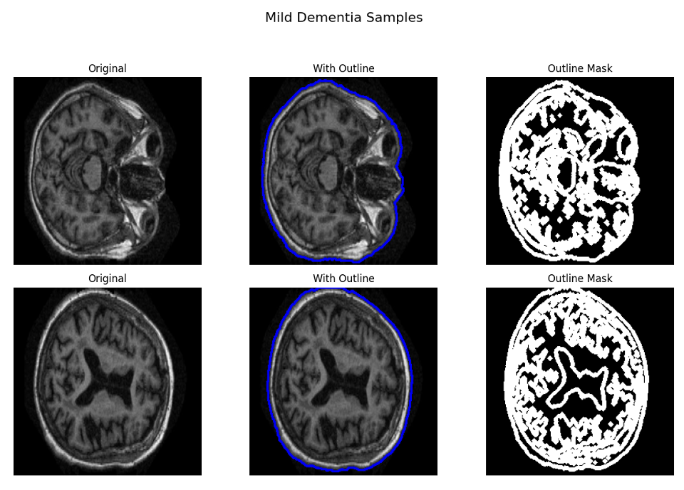
ROI extraction — original, brain outline, and binary mask — Figure 6 — ROI extraction. For each scan we detect the brain outline and derive a binary mask that focuses the discriminator on the relevant region.

The improvement is measurable. At epoch 15 on the Very Mild→Mild transition, the ROI-guided model beat the baseline on every metric we tracked — pixel error, signal quality, structural and perceptual similarity, and distribution realism:

Metric	Without ROI	With ROI	Better
MSE	0.0378	0.0326	lower ↓
PSNR (dB)	14.33	14.93	higher ↑
SSIM	0.3295	0.3330	higher ↑
LPIPS	0.3191	0.3092	lower ↓
FID	39.99	30.94	lower ↓

ROI-guided generation — original, generated, and difference map — Figure 7 — ROI-guided output: original scan, generated next-stage scan, and their difference map highlighting where the model introduced change.

ROI guidance cut FID from 39.99 → 30.94 — roughly a 23% gain in realism — and lifted PSNR by 0.6 dB, with SSIM and LPIPS improving in lockstep. Concentrating the adversarial signal on the brain itself, rather than the background, is what made the generated scans sharper and more anatomically faithful.

Deployment & Experiment Tracking

The system ships as a Flask web application: a user uploads an MRI, the classifier identifies the current stage, the GAN chain generates the remaining progression, and the original and synthesized scans are rendered side by side. The app is containerized with Docker for one-command reproducible deployment (it runs live on Render), and inference uses Apple MPS/CUDA acceleration when present.

Training is fully tracked with MLflow under a dedicated Alzheimers_Classifier experiment: every run logs its hyperparameters (batch size, both learning rates, epoch counts, image size), per-epoch train/validation loss and accuracy for both phases, and registers the resulting model. That makes runs directly comparable in the MLflow UI and the whole experiment reproducible rather than a one-off result buried in a notebook.

Engineering Challenges Solved

Extreme class imbalance (~138:1): healthy scans swamp late-stage ones. Addressed with transfer learning plus minority upsampling for GAN training, and — crucially — reporting macro-F1 alongside accuracy so the minority stages can't hide behind the majority.
Subtle inter-stage differences: adjacent stages are structurally similar (confirmed by SSIM and the mean-difference maps). Tackled with intensity normalization and an ROI-aware discriminator that focuses learning on the regions that actually change.
Two-phase fine-tuning, not blind training: fine-tuning a 17M-parameter backbone from the start would wreck the ImageNet features. Freezing first, then unfreezing at a low learning rate, is what unlocked the 78%→98% jump.
Encoder–decoder bottleneck: compressing a scan to 256 feature maps and reconstructing it risks losing fine detail. ROI guidance and pixel-range normalization (Tanh + [-1,1]) mitigated the information loss.
Chaining generators without drift: feeding one GAN's output into the next can compound artifacts, so each transition is a dedicated, separately-trained model rather than one generator asked to do everything.
Reproducibility & hardware portability: MLflow tracking plus Docker, with an MPS/CUDA/CPU device fallback, so the project trains and serves on a laptop or a cloud box without code changes.

Tech Stack

Deep learning: PyTorch & torchvision (EfficientNetB4 transfer learning, custom DCGAN generator/discriminator).
Data & analysis: OASIS MRI dataset, OpenCV, scikit-image (SSIM), NumPy, pandas, Matplotlib & Seaborn for EDA.
Generation metrics: MSE, PSNR, SSIM, LPIPS, and FID for evaluating synthesized scans.
Serving: Flask web app with HTML/CSS/JS front end, MPS/CUDA-accelerated inference.
MLOps: MLflow (experiment tracking & model registry), Docker, Git LFS for model weights, deployed on Render.

Outcomes & Impact

Built a complete diagnosis-and-prognosis system — staging classifier plus generative progression — over 86,437 OASIS MRI slices.
Achieved 98% accuracy and 0.98 macro-F1 across all four stages on a 2,048-image held-out set, holding 0.95 F1 even on the hard Very Mild class.
Trained three stage-transition DCGANs and chained them into a coherent, stage-by-stage progression visualizer.
Improved generation quality with ROI guidance — FID 39.99 → 30.94 (~23% better) and +0.6 dB PSNR, with SSIM and LPIPS improving too.
Shipped the whole thing as a Dockerized Flask app with MLflow tracking and a public live demo.

Conclusion

This project is where I learned to make generative models and transfer learning work together on a genuinely messy, imbalanced medical dataset — and to be honest about what the numbers mean. The standout lessons were practical: how a two-phase fine-tuning schedule converts a frozen 78% into a fine-tuned 98%, how an encoder–decoder bottleneck quietly eats detail in GAN outputs, and how focusing the discriminator on a region of interest measurably improves realism. The same recipe — classify the present state, then generate the likely future — extends naturally to other progressive conditions such as tumor growth or retinal disease, where seeing the trajectory is as valuable as naming the stage.